Projects

Fourier analysis of double-slit interference patterns, demonstrating wave-particle duality and quantum mechanics principles. It uses the split-step Fourier method: apply half the potential $e^{-iV \Delta t/2}$, transform to Fourier space for the kinetic step $e^{-iK \Delta t}$ where $K = \frac{1}{2}(k_x^2 + k_y^2)$, then transform back and apply the other half.

This simulation visualizes two-dimensional wave propagation on a grid with customizable Gaussian/Lorentzian initial bumps & region-specific wave speeds. Combined with the discrete Laplacian operator, they lead to the evolving 3D hat-shaped surface seen here. The update loop uses $a = c^2 \nabla^2 u$, $v \mathrel{+}= a \cdot dt$, $u \mathrel{+}= v \cdot dt$, and the hat comes from subtracting two Lorentzians $L(\gamma, A) = \frac{A}{1 + (r/\gamma)^2}$.

Zernike polynomials are a set of mathematical shapes used to describe optical aberrations - deviations from a perfect wavefront that cause imperfections in lenses and mirrors, like blur, stretched images, or comet-like smearing. Each polynomial $Z_n^m(r,\theta)$ captures a specific type of distortion. This animation sweeps through different aberration modes and shows how each one warps the point spread function (PSF) - what a single point of light looks like after passing through the optic. The wavefront is built from $W = \sum a_j Z_j(r,\theta)$ with oscillating amplitudes, then Fourier-transformed to get the PSF.

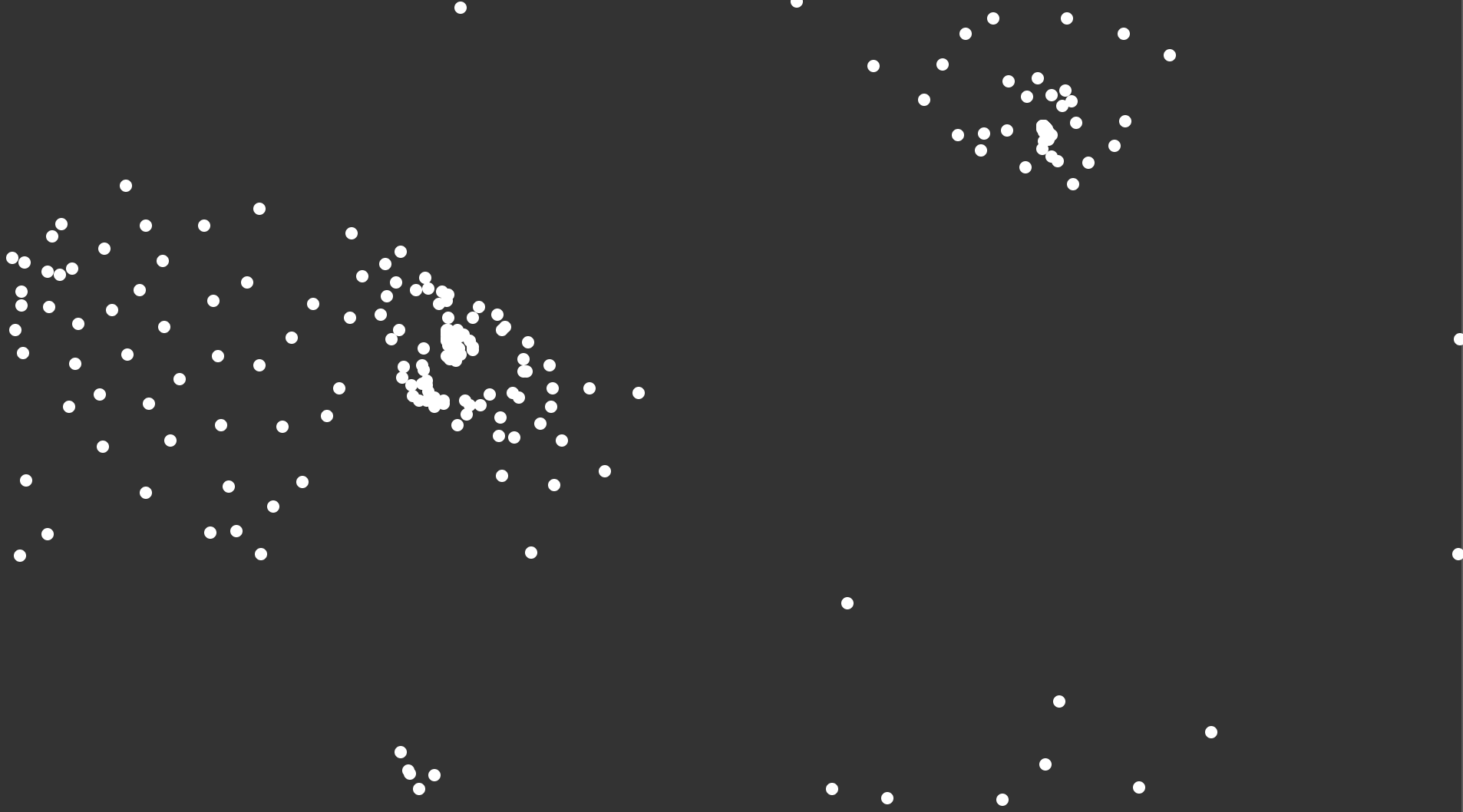
Just like birds moving around in the sky, this simulation shows how each boid decides based only on its nearby neighbors - a classic example of emergent behavior. Each boid follows three simple rules: separation (avoid crowding), alignment (steer toward average heading), and cohesion (move toward the group's center). The resulting acceleration is $\mathbf{a} = w_s \mathbf{s} + w_a \mathbf{a} + w_c \mathbf{c}$, where each force is computed locally within a perception radius. By tweaking these weights, the boids reorganize into smooth, lifelike flocks - proving that simple local rules can produce complex global patterns.

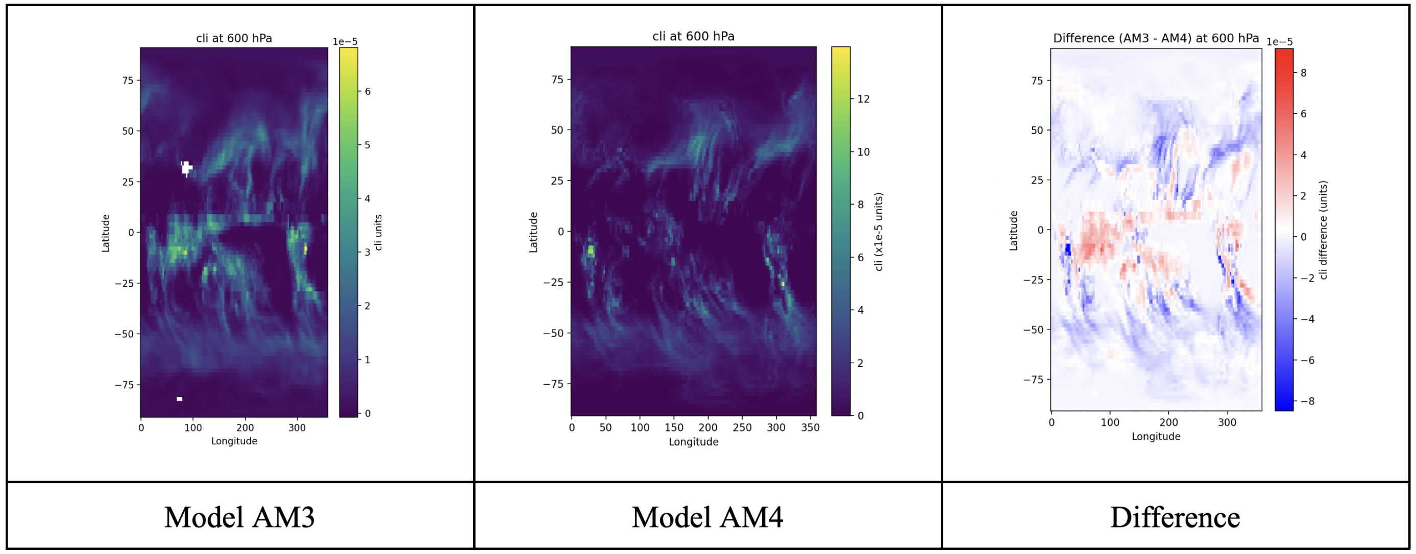
This loads two different GFDL AM3 and AM4 NetCDF outputs for cloud ice (cli) in Jan 2009, computes their differences, and demonstrates three different (but complementary) comparisons: 1) latitude–longitude maps at multiple pressure levels 2) latitude-pressure zonal‐mean difference plots, and 3) vertical profile difference charts. Also my first project in modeling & data comparison!

Discovered by meteorologist Edward Lorenz in 1963, this system is governed by three coupled ODEs: $\dot{x} = \sigma(y-x)$, $\dot{y} = x(\rho-z) - y$, $\dot{z} = xy - \beta z$. With parameters $\sigma = 10$, $\rho = 28$, $\beta = 8/3$, the system enters its chaotic regime. I integrate numerically using RK4 from $(x_0, y_0, z_0) = (0.1, 0, 0)$, discarding transients to reveal the iconic "butterfly wing" attractor.

Like a tug-of-war between gravity and inertia, this traces one mass sliding on a frictionless table tied to another hanging mass. Changing the initial stretch slider makes the orbit swell and shrink, with neither gravitational pull nor angular momentum ultimately winning over one another. 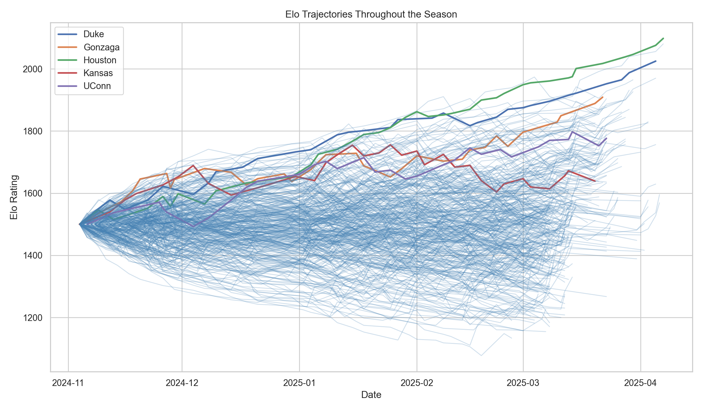This was inspired in part by Problem 1.26 in Cahn, which can be solved with generalized coordinates in Lagrangian mechanics.

This NCAA basketball model uses logistic regression, Bayesian shrinkage, and linear least squares to predict true team strengths from three models: Elo, Bradley-Terry, and Massey. The Elo update is $R' = R + K(S - E)$ where $E = \frac{1}{1 + 10^{(R_B - R_A)/400}}$, Bradley-Terry estimates $P(A \text{ beats } B) = \frac{p_A}{p_A + p_B}$, and Massey solves $Mr = p$ for ratings. A Tikhonov-regularized logistic layer $P = \sigma(\beta^T x)$ with $\|\beta\|^2$ penalty converts features to win probabilities. Validation includes LogLoss, Brier score, AUC, and calibration curves.